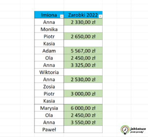
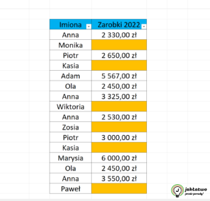
Do you want to automatically highlight empty/blank cells in a spreadsheet with color? There is a quick way to do it. Just use conditional formatting. This will automatically change the color depending on whether or not a value appears in the cell.

1. Open the spreadsheet on your computer;
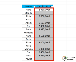
2. Select the range for which you would like to implement the conditional formatting mechanism (we omit row and column headers). You can also use the keyboard shortcut CTRL+SHIFT+Down arrow – a very quick way and useful when working with large amounts of data;
   
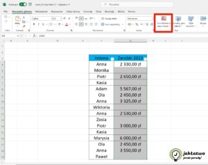
3. Go to the top navigation bar and then click on the “Main Tools” tab;
   
4. In the “Styles” area, click on the “Conditional Formatting” option;
   
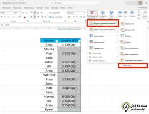
5. Click on the “Cell highlight rules” category and then select the “More rules” command;
   
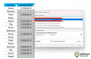
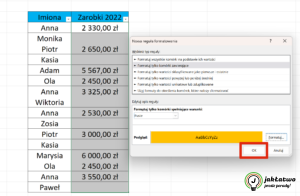
6. A dialog box will appear. Select the type of rule. You should check “Format only containing cells”;
   
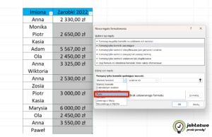
7. Select “Blank” from the drop-down list, which is located in the “Format only cells that meet the conditions” area;
   
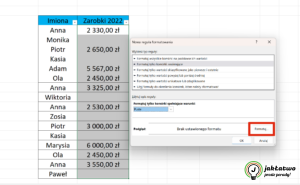
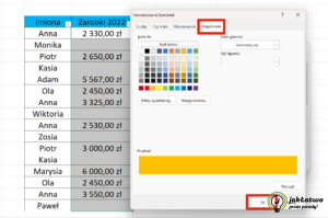
8. Click on the “Format” button and then go to the “Fill” tab and indicate the color to appear in the cells if the cells do not contain any value. Confirm by clicking on the “OK” button;
   
9. If you want the color to appear in cells containing values, you follow the same procedure as for blank cells (steps 1-6 and 8) with the difference (step 7) that you select “Non-empty” from the drop-down list that is located in the “Format only cells that meet conditions” area.